We’ve just seen that solutions of one-dimensional systems behave rather trivially. But dependence on parameters adds spice because qualitative changes in the behavior of solutions can occur. These changes are called bifurcations.
This chapter aims at introducing a few examples and not developing the full theory. We’ll explore additional types of bifurcations when we step up to two- and three-dimensional systems.
The basic setting is a one-dimensional differential equation $\dot{x}=f_\mu(x)$, where $\mu$ is a real parameter. We expect that varying $\mu$ can cause the emergence or destruction of equilibria and also affect their stability.
A model of a fishery with a saddle-node bifurcation
The equation $\dot{x}=rx\left(1-\frac{x}{K}\right)-h$ provides an oversimplified mode l of a fishery. In the absence of fishing, the population is assumed to grow according to the logistic equation. The effects of fishing are modeled by the term $-h$, which says that fish are caught at a constant rate $h>0$, independent of their abundance $x$. This assumes that the fishermen catch the same number of fish every day, without worrying about fishing the population dry.
A priori, we have three parameters, but the system can be rewritten in dimensionless form as
$$ \dot{x}=x(1-x)-\mu $$
by a suitable rescaling. We already mentioned nondimensionalization when we discussed Volterra’s model for sharks and sardines in the first chapter. We see here the usefulness of this procedure since we see that, as a matter of fact, the system depends only a single (dimensionless) parameter.We can observe the following behaviors.
The fixed points are the solutions of the quadratic equation $x(1-x)-\mu=0$. There are two equilibria if $\mu\in (0,1/4)$, one is stable and the other is unstable. When $\mu=1/4$, these equilibria coalesce into a ‘half-stable’ fixed point that corresponds to the unique solution of the quadratic equation. As soon as $\mu>1/4$, this fixed point vanishes and there no equilibria at all.
We say that a bifurcation occurred at $\mu=\frac{1}{4}$. This bifurcation is called a saddle-node bifurcation. (The reason for that name will become self-evident when we see a completely analogous bifurcation in dimension two.) It is the basic mechanism by which fixed points are created and destroyed: as a parameter is varied, two fixed points move toward each other, ‘collide’, and mutually ‘annihilate’.
An example of transcritical bifurcation
There is something silly about the previous model because the population can become negative. A better model would have a fixed point at zero population for all values of the parameter. The simplest way to achieve this is to set
$$ \dot{x}=x(1-x)-\mu x $$
where $\mu>0$ represents the fraction of the population that fishermen catch per unit time. Letting $r=1-\mu$ this equation becomes$$ \dot{x}=rx-x^2. $$
It looks like the logistic equation but, forgetting about its interpretation as a population model, we now allow $x$ and $r$ to be either positive or negative. Regardless of the value of $r$, $0$ is a fixed point but we are going to see that it changes its stability as $r$ is varied, as the following experiment shows.
We observe that, for $r<0$, there is an unstable fixed point $\bar{x}=r$ and the origin $0$ is a stable one. As $r$ increases, the unstable fixed point approaches the origin and coalesces with it when $r=0$. Finally, when $r>0$, the origin becomes unstable, and $\bar{x}=r$ is now (asymptotically) stable. We can say that an exchange of stabilities has taken place between the two fixed points. This bifurcation occurred at $r=0$. The example we consider may seem particular but it is not in fact: close to a transcritical bifurcation, the dynamics looks like $\dot{x}=rx-x^2$.
An insect outbreak model
We end this chapter by a biological example of bifurcation and catastrophe, namely a model for the sudden outbreak of an insect called the spruce budworm. When an outbreak occurs, this insect can actually defoliate and kill the balsam fir in forests of eastern Canada in about four years. The simplest version for a model of the interaction between budworms and the forest relies on a separation of time scales: the budworm population evolves on a much faster time scale than the trees. Thus, as a first approximation, the forest variables may be treated as constants. The proposed model for the budworm dynamics is
$$ \dot{x}=\rho x\left( 1-\frac{x}{\kappa}\right)-\frac{\beta x^2}{\alpha^2+ x^2}, $$
where the parameters $\alpha,\beta,\kappa,\rho$ are positive parameters. In the absence of predators, the budworm population density $x(t)$ is assumed to grow logistically with growth rate $\rho$ and carrying capacity $\kappa$. The carrying capacity depends on the amount of foliage left on the trees but we treat it here as fixed, as mentioned above. The term $\frac{\beta x^2}{\alpha^2+ x^2}$ represents the death rate due to predation, chiefly by birds.
The specific form for the death rate takes into account, in the simplest way, the following behaviors. There is almost no predation when budworms are scarce; the birds search for food elsewhere. But, when the population density exceeds a certain critical level $x=\alpha$, the predation turns on sharply and then saturates.
You can now ask: what do you mean by an outbreak? Before answering this question, it is convenient to recast the model into a dimensionless form, as we did before for simpler models. Indeed, the model has four (positive) parameters: $\rho,\kappa,\alpha$ and $\beta$. If you start playing the game of rescaling the equation, it will be clear that there are various ways of doing it. It turns out, after some trial and error, that a very convenient choice is to get rid of the parameters in the predation term. After some algebra, this gives the dimensionless model
$$ \dot{x}=rx\left(1-\frac{x}{K}\right) - \frac{x^2}{1+x^2}\, \cdot $$
Analysis of fixed points.
We always have the fixed point $x=0$ and it is not difficult to check that it is always unstable by applying the derivative test. Intuitively, this is not surprising since for very small $x$, we approximately have $\dot{x}\approx rx$. The other possible fixed points of the equation are given by the solutions of the equation
$$ g(x)=h(x) $$
where$$ g(x)=r\left(1-\frac{x}{K}\right)\quad \text{and}\quad h(x)=\frac{x}{1+x^2}\, \cdot $$
Notice that the function $h$ is independent of the parameters; only the function $g$, whose graph is a straight line, moves when $r$ and $K$ are varied. This is due to our choice of nondimensionalization.
As the experiments shows, if $K$ is sufficiently small, there is exactly one intersection for any $r>0$. But, for large $K$, we can have one, two, or three intersections, depending on the value of $r$. We can observe that, when we are in the range of parameters for which there are three intersections, as we decrease $r$ with $K$ fixed, the fixed points $b$ and $c$ approach each other and eventually coalesce. This is the signature of a saddle-node bifurcation. After the bifurcation, there is only one remaining fixed point (in addition to $0$, of course). Another way of varying the parameters is to fix $K$ and, starting for a small $r$, we observe that $a$ and $b$ can collide and annihilate as $r$ is increased.
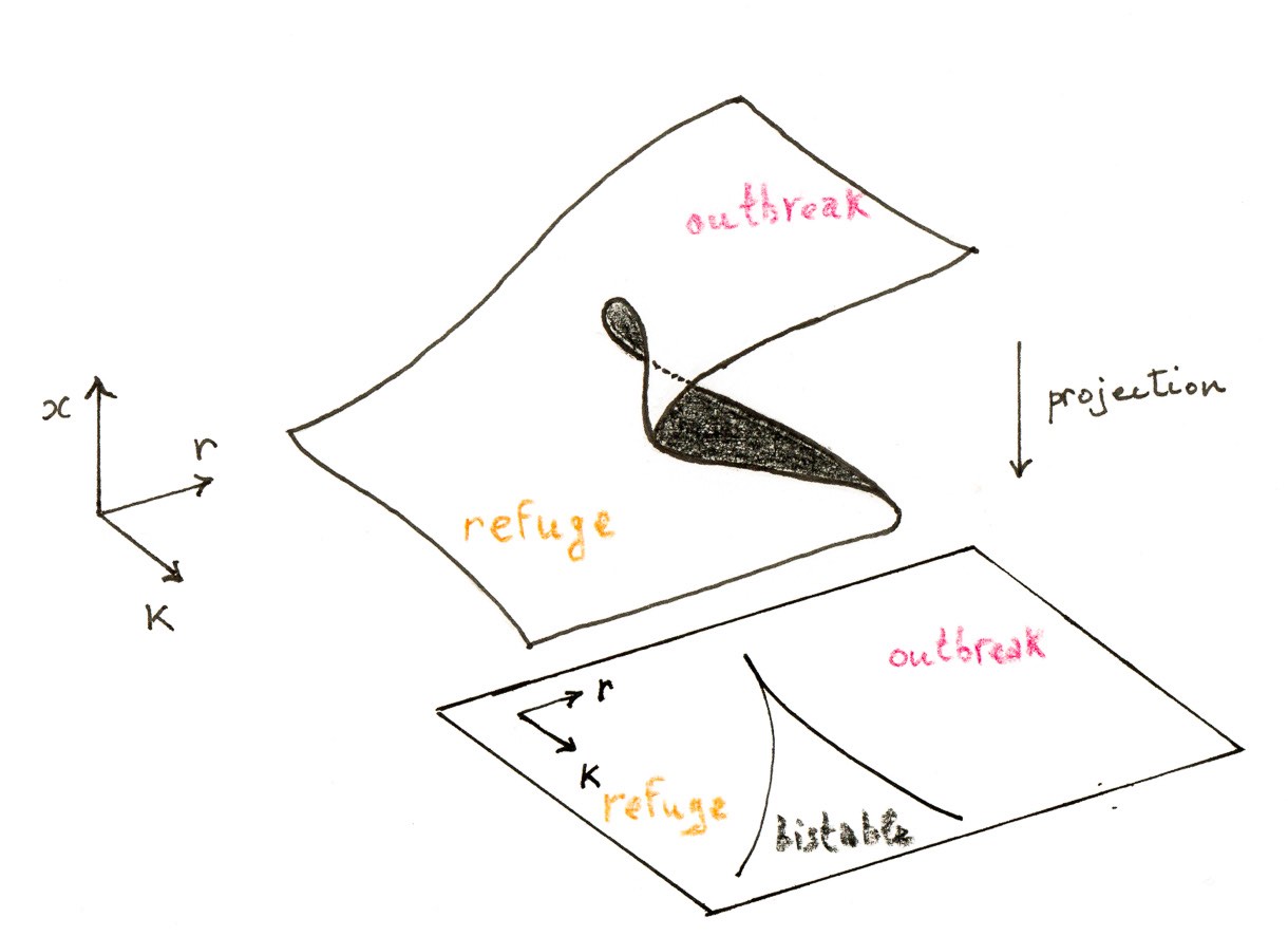
The experiments also shows how the stability of the fixed points change as $r$ and $K$ are varied. For the values corresponding to three fixed points, the smaller stable fixed point $b$ is called the refuge level of the budworm population, while the larger stable fixed point $c$ is the outbreak level. From the point of view of pest control, one would like to keep the population density at $a$ and away from $c$. The fate of the system is determined by the initial condition $x_0$. An outbreak occurs if and only if $x_0>b$; the unstable fixed point $b$ plays the role of a threshold.
Another more interesting scenario leading to an outbreak is by a saddle-node bifurcation. Indeed, imagine that now that $r$ and $K$ drift in such a way that the fixed point $a$ disappears; then the population will jump suddenly to the outbreak level $c$. The situation is in fact even worse because there is a so-called hysteresis effect: even if the parameters are restored to their values before the outbreak, the population will not drop back to the refuge level!
The richness of this simple model is quite remarkable. It illustrates the fact that we must not underestimate one-dimensional models when bifurcations can occur.