The Rössler attractor

In 1976, Rössler constructed the following three-dimensional system

$$ \begin{cases} \dot{x}=-y-z\\ \dot{y}=x+a y\\ \dot{z} = b+z(x-c) \end{cases} $$

where $a,b$, and $c$ are parameters. Rössler was looking for a system behaving like the Lorenz system, but easier to analyze. Note that the only nonlinear term appears in the $\dot{z}$ equation and is quadratic. Note also that, if $z=0$, we get a linear system in the $xy$-plane. As the parameters vary, this simple system can display a wide range of behavior.

It is easy to check that there are at most two fixed points, namely

$$ \left(\, \frac{c\pm \sqrt{c^2-4ab}}{2},\, \frac{-c\mp \sqrt{c^2-4ab}}{2a},\, \frac{c\pm \sqrt{c^2-4ab}}{2a}\, \right) $$

which exist provided that $c^2\geq 4ab$.

Let’s start with Rössler’s values for the parameters:

$$ a=0.2,\thinspace b=0.2,\thinspace c=5.7. $$

We can observe that a solution within the attractor follows an outward spiral close to the $xy$-plane around one of the fixed points. Once the solution spirals out enough, the second fixed point influences the trajectory of the solution in that it can cause a rise and twist in the $z$-dimension. Sensitive dependence on initial conditions manifest clearly, as the next experiment shows.

You can explore the behavior of solutions of the Rössler system as parameters change.

The Rössler system has an incredibly rich behavior as the parameters are varied. Let’s tell a little part of the story.

You can for instance fix $b$ at $0.2$ and $c$ at $5.7$, and change $a$. You can then observe the following behaviors:

• $a=0.1$: unit cycle of period $1$;
• $a=0.2$: the Rössler attractor;
• $a=0.3$: chaotic attractor, M\"obius strip-like;
• Increasing $a$ further gives a chaotic attractor similar to the case $a=0.3$, it looks more and more chaotic.

You can also take $a=b=0.2$ and make $c$ increasing from $2.5$ to $10$. You will observe ‘windows’ of periodicity interspersed with ‘windows’ of chaos (aperiodicity).

• $c=2.5$: solutions go end up on an attractor which is a limit cycle;
• $c=3$: the limit cycle is twisted and still attractive. Looking at the time series plots, that is $x(t)$, $y(t)$ or $z(t)$, we observe that there are two distinct sets of peaks and troughs. Looking at the projection in the $xy$-plane, this means that the corresponding solution (once it is on the limit cycle) makes two loops before it takes back the same values.
• $c=4$: we observe a further twist of the attractive limit cycle which corresponds to four distinct sets of peaks and troughs.
• $c=4.2$: we have yet another twist which corresponds to eight distinct sets of peaks and troughs. This is the beginning of a period-doubling cascade, that is, a sequence of period-doubling bifurcations.
• As $c$ increases a bit, we observe a chaotic behavior. In fact, with a higher resolution, one could see further period doublings (in fact, infinitely many) in a finite size interval.
• As $c$ goes on increasing, we can observe the reappearance of an attractive limit cycle for a small interval of parameters. Increasing $c$, we can observe a new period-doubling cascade leading to chaos which takes place in a shorter interval than for the previous period-doubling cascade.

A concise and striking way of visualizing the phenomena we’ve just described is to draw a bifurcation diagram.

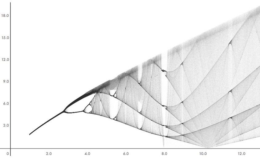
There are various ways of drawing such a diagram. Here we make it as follows. Forget about $z(t)$ and record the positive values of $x(t)$ when $y(t)$ goes through the threshold $y=0$. Of course, we have to let aside the transient behavior. If for a given value of $c$ there are, say, four points, this means that we have a limit cycle and that the corresponding projected periodic solution on the $xy$-plane makes four loops before it takes back the same values.