We previously said that most differential equations cannot be solved explicitly. This is not completely true : linear differential equations can be analysed thoroughly. Most models in physics, biology, etc are nonlinear differential equations, but linear ones play an important role in the classification of their fixed points, as we shall see later on.
Definition
A two-dimensional linear system is a system of the form
$$ \begin{cases} \dot{x}= ax+by\\ \dot{y}= cx+dy \end{cases} $$
where $a,b,c,d$ are parameters. In vector notation this is written more compactly in matrix form as$$ \dot{\boldsymbol{x}}=A\boldsymbol{x} $$
where$$ A= \begin{pmatrix} a & b\\ c & d \end{pmatrix} \hspace{0.5cm}\text{and}\hspace{0.5cm} \boldsymbol{x}= \begin{pmatrix} x\\ y \end{pmatrix}\, . $$
Such systems are the natural two-dimensional version of the scalar equation $\dot{x}=ax$ which is the first one that appeared in this ebook. We say that it is linear because if $\boldsymbol{x}_1$ and $\boldsymbol{x}_2$ are solutions, then so is any linear combination $c_1 \boldsymbol{x}_1+ c_2 \boldsymbol{x}_2$. Notice that $\dot{\boldsymbol{x}}=\boldsymbol{0}$ when $\boldsymbol{x}=\boldsymbol{0}$, so $\bar{\boldsymbol{x}}=\boldsymbol{0}$ is always a fixed point for any choice of $A$.Examples
Back to the harmonic oscillator.
We already met an example of a two-dimensional linear differential equation, namely the harmonic oscillator. Recall that it is a particle of mass $m$ moving on the $x$-axis subject to the force $f(x)=-kx$. As we saw, the equation of motion $\ddot x=-kx$ can be represented as a linear two-dimensional system $\dot{\boldsymbol{x}}=A\boldsymbol{x}$ with
$$ A= \begin{pmatrix} 0 & 1\\ -\omega^2 & 0 \end{pmatrix} $$
where $\omega^2=\frac{k}{m}$. We can add a friction force of the form $-\epsilon \dot{x}$, where $\epsilon>0$, which gives a linear two-dimensional system with$$ A= \begin{pmatrix} 0 & 1\\ -\omega^2 & -\epsilon \end{pmatrix}. $$
We see that, when $\epsilon=0$, all trajectories are closed and encircle the origin (the unique fixed point) which is called a center. When $\epsilon>0$, trajectories are no more closed: the solutions spiral towards the origin.
Circuit theory.
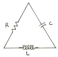
Our next example comes from circuit theory, more precisely a series RLC circuit, where $R$ stands for resistor, $L$ for inductor, and $C$ for capacitor. In this model, the resistor is alone responsible for energy dissipation, while the inductor and the capacitor are idealized as being able to store energy without dissipation.
Assuming that the circuit has a power source displaying a voltage that is constant in time, we can apply Kirchhoff’s current law, Faraday’s law, and Ohm’s law to get the second-order differential equation
$$ L \ddot{I}+R\dot{I}+\frac{I}{C}=0 $$
where $I(t)$ is the current in the circuit and $L,C>0$ and $R\geq 0$ are parameters. Ohm’s law says that the voltage across the resistor is proportional to the current, the constant of proportionality being $R$. This relationship makes the system linear. Many resistors obey Ohm’s law. (Observe that when $R=0$ we get an equation that is formally the same as the one for the harmonic oscillator.) We can rewrite the equation as a two-dimensional linear differential equation by setting $x=I$ and $y=\dot{x}$. This gives$$ \begin{cases} \dot{x}= y\\ \dot{y}= - \frac{1}{L C}\thinspace x-\frac{R}{L} y \end{cases} $$
thus$$ A= \begin{pmatrix} 0 & 1\\ - \frac{1}{L C} & -\frac{R}{L} \end{pmatrix}. $$
By the way, we observe that the system obtained for the RLC circuit has exactly the same form as the one describing a damped harmonic oscillator if we identify $\frac{1}{L C}$ with $\omega^2$ and $\frac{R}{L}$ with $\epsilon$. Indeed, $R=0$ corresponds to an ideal circuit in which there would not be energy dissipation by Joule’s effect.
An abstract example.
We now consider the linear system
$$ \begin{cases} \dot{x}= a x\\ \dot{y}= -y \end{cases} $$
where $a\in\mathbb{R}$ is a parameter. In vector notation, this means that $\dot{\boldsymbol{x}}=A\boldsymbol{x}$ with$$ A= \begin{pmatrix} a & 0\\ 0 & -1 \end{pmatrix}. $$
The two equations are uncoupled in the sense that there is no $x$ in the $y$-equation and vice versa. This implies that each equation may be solved separately. We easily get$$ x(t)=x_0\ e^{at},\thinspace y(t)=y_0\ e^{-t}. $$
The geometry of trajectories in the neighborhood of the origin, which is a fixed point for any value of $a$, can be explored with the following interactive digital experiment.
Let us comment on what we observe.
Of course, we know that $y(t)$ decays exponentially with $t$ whatever is the value of $a$. When $a<0$, $x(t)$ also decays exponentially and so all trajectories approach the origin as $t\to+\infty$. However, the direction of approach depends on the size of $a$ compared to $-1$.
When $a<-1$, $x(t)$ decays more rapidly than $y(t)$. The solutions approach the origin tangent to the slower direction, that is, the $y$-direction. The fixed point $\bar{\boldsymbol{x}}=\boldsymbol{0}$ is called an nodal sink.
When $a= - 1$, we have $y(t)/x(t)=y_0/x_0$ for all $t$, and so all trajectories are straight lines through the origin. This is a very special case since the decay rates in the two directions are exactly equal.
When $a\in\, ]-1,0\, [$, we also get a nodal sink but now the solutions approach the origin along the $x$-direction, which is the more slowly decaying direction in this case.
When $a=0$, the system is quite degenerate: $x(t)=x_0$ for all $t$, so there is an entire line of fixed points, namely the whole $x$-axis.
Finally when $a>0$, $\bar{\boldsymbol{x}}$ becomes unstable, due to the exponential growth in the $x$-direction. We see that all solutions deviate from the origin and head out to infinity, except those starting on the $y$-axis wich converge to it. Here $\bar{\boldsymbol{x}}=\boldsymbol{0}$ is called a saddle. The $y$-axis is called the stable manifold of the saddle point $\bar{\boldsymbol{x}}$, defined as the set of initial conditions $\boldsymbol{x}_0$ such that $\boldsymbol{x}(t)=\bar{\boldsymbol{x}}$ as $t\to+\infty$. Likewise, the unstable manifold of $\bar{\boldsymbol{x}}$ is the set of initial conditions such that $\boldsymbol{x}(t)=\bar{\boldsymbol{x}}$ as $t\to-\infty$. Here it is the $x$-axis.
We can also observe what happens when we reverse time: attractiveness is changed into repulsiveness, and for the saddle point the stable manifold becomes unstable whereas the unstable one becomes stable.
Classification of possible phase portraits
Eigenvalues, eigenvectors & eigensolutions.
The previous example has the special feature that two of the entries in the matrix $A$ are zero, making the system uncoupled. Of course, we want to study the general case and get a classification of all possible phase portraits. Inspired by that example, we can figure out how to proceed. Indeed, the $x$ and $y$ axes play a crucial geometric role: they determine the direction of the trajectories as $t\to \pm \infty$. They also contain special straight-line trajectories: a solution starting on one of the coordinate axis stayed on that axis forever, and exhibit simple exponential growth or decay along it. What is the analog in the general case? Well, we would like to find the analog of the straight-line trajectories, that is, we look for solutions of the form
$$ \boldsymbol{x}(t)=e^{\lambda t}\boldsymbol{v} $$
where $\boldsymbol{v}\neq \boldsymbol{0}$ is some fixed vector to be determined, and $\lambda$ is a growth rate, also to be determined. If such solutions exist, they correspond to solutions moving exponentially fast along the line spanned by the vector $\boldsymbol{v}$.Let us find the conditions on $\boldsymbol{v}$ and $\lambda$: we subtitute $\boldsymbol{x}(t)=e^{\lambda t}\boldsymbol{v}$ into $\dot{\boldsymbol{x}}=A\boldsymbol{x}$, and get, after cancelling the nonzero scalar factor $e^{\lambda t}$:
$$ A\boldsymbol{v}=\lambda \boldsymbol{v}. $$
This equation says that the wanted straight line solutions exist if $\boldsymbol{v}$ is an eigenvector of $A$ with corresponding eigenvalue $\lambda$. A solution of the form $\boldsymbol{x}(t)=e^{\lambda t}\boldsymbol{v}$ is called an eigensolution.If you know basic linear algebra, you should not be surprised by the following considerations. In general, the eigenvalues of a matrix $A$ are given by the so-called charateristic function $\text{det}(A-\lambda\mathbb{1})=0$, where $\mathbb{1}$ is the identity matrix ($1$’s on the diagonal entries and $0$’s elsewhere). For $2\times 2$ matrix, this equation is simply
$$ \text{det} \begin{pmatrix} a-\lambda & b\\ c & d-\lambda \end{pmatrix}=0, $$
that is,$$ \lambda^2 -\text{tr}(A)\thinspace\lambda+\text{det}(A)=0 $$
where$$ \text{tr}(A)=a+d,\thinspace \text{det}(A)=ad-bc. $$
The solutions of the characteristic equation are$$ \lambda_1=\frac{\text{tr}(A)+\sqrt{\Delta}}{2},\thinspace\thinspace \lambda_2=\frac{\text{tr}(A)-\sqrt{\Delta}}{2} $$
where$$ \Delta=\text{tr}(A)^2-4\text{det}(A) $$
is the discriminant of the above quadratic equation.We also observe that, by definition of $\lambda_1$ and $\lambda_2$, we have
$$ (\lambda-\lambda_1)(\lambda-\lambda_2)=\lambda^2 -\text{tr}(A)\thinspace\lambda+\text{det}(A)=0 $$
giving by identification$$ \text{det}(A)=\lambda_1\lambda_2, \thinspace\thinspace\text{tr}(A)=\lambda_1+\lambda_2. $$
The typical situation is for the eigenvalues to be distinct: $\lambda_1\neq \lambda_2$. It follows from a general theorem of linear algebra that the corresponding eigenvectors $\boldsymbol{v}_1$ and $\boldsymbol{v}_2$ are linearly independent, and hence span the entire plane.
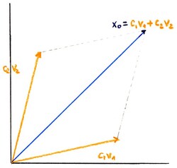
In particular, an initial condition $\boldsymbol{x}_0$ can be written as a linear combination of eigenvectors, say $\boldsymbol{x}_0=c_1\boldsymbol{v}_1+c_2\boldsymbol{v}_2$. Hence we can write down the general solution for $\boldsymbol{x}(t)$: it is
$$ \boldsymbol{x}(t)=c_1\ e^{\lambda_1 t}\boldsymbol{v}_1 + c_2\ e^{\lambda_2 t}\boldsymbol{v}_2. $$
First, it is a linear combination of solutions to $\dot{\boldsymbol{x}}=A\boldsymbol{x}$, and hence itself a solution. Second, it satisfies the initial condition $\boldsymbol{x}(0)=\boldsymbol{x}_0$, and so by the existence and uniqueness theorem stated in the preceding section, it is the only solution.Summarizing view of all phase portraits.
The next step is to classify all possible phase portraits as the entries of $A$ vary. In the following interactive digital experiment, we display three views that interact between themselves: the phase plane, the eigenvalues in the complex plane, and the $(\text{tr}(A),\text{det}(A))$ plane. You can either tune the entries of $A$ and see the resulting phase portrait, together with the corresponding eigenvalues and the the corresponding value for $(\text{tr}(A),\text{det}(A))$. But you can also move the eigenvalues and see the resulting effect, or act in the $(\text{tr}(A),\text{det}(A))$ plane to see what happens to the phase portrait and the eigenvalues.
The following picture is a visual summary of all possible phase portraits, together with the names given to the fixed point $\bar{\boldsymbol{x}}=\boldsymbol{0}$ in the different cases that occur.

Let us come back to the examples presented above in the light of what we have done.\
We see that the origin is a center for the harmonic oscillator. In this case, $\text{det}(A)=\omega^2$ and $\text{tr}(A)=0$.
For the RLC circuit we have
$$ \text{det}(A)=\frac{1}{L C}>0,\thinspace\thinspace\text{tr}(A)=-\frac{R}{L}\leq 0,\thinspace\thinspace\text{and}\thinspace\thinspace \Delta=\frac{R^2 C-4L}{L^2C}. $$
Thus, in the $(\text{tr}(A),\text{det}(A))$ plane, we are in the quadrant $\{\text{tr}(A)\leq 0,\text{det}(A)>0\ \}$ (the second quadrant). If $R=0$ the origin is a center. If $R>0$ then the origin is either a nodal sink if $R^2 C-4L>0$, or it is a spiral sink if $R^2 C-4L<0$. When $R^2 C-4L=0$ we have a degenerate nodal sink.For the third example we have
$$ \text{det}(A)=-a, \thinspace\thinspace\text{tr}(A)=a-1. $$
When $a>0$, the origin is a saddle. When $a<0$, it is a nodal sink.Understanding more about the classification.
The previous interactive digital experiment and the associated picture gather in a compact way all informations about the behavior of solutions and the geometry of the corresponding trajectories of two-dimensional linear differential equations. In particular, we can see how solutions are attracted or repelled by the origin. Here we analyse what is behind these pictures from a mathematical viewpoint. The impatient reader can jump over this section and come back later on.
All the information we need is contained in the following formulas that we derived above:
$$ \lambda_{1,2}=\frac{\text{tr}(A)\pm\sqrt{\text{tr}(A)^2-4\text{det}(A)}}{2} \thinspace,\thinspace\thinspace \text{det}(A)=\lambda_1\lambda_2, \thinspace\thinspace \text{tr}(A)=\lambda_1+\lambda_2. $$
- If $\text{det}(A)<0$, this means that the eigenvalues are distinct, real and have opposite signs. The eigensolution corresponding to the negative eigenvalue decays exponentially. The eigensolution corresponding to the positive eigenvalue grows exponentially. This means that the origin is a saddle.
- If $\text{det}(A)>0$, the eigenvalues are either real with the same sign (nodal sinks/sources), or complex conjugate (spiral sinks/sources and centers). Nodal sinks/sources satisfy $\text{tr}(A)^2-4\text{det}(A)>0$ and spiral sinks/sources satisfy $\text{tr}(A)^2-4\text{det}(A)<0$. The difference between sinks and sources is given
by the sign of $\text{tr}(A)$: when $\text{tr}(A)<0$, both eigenvalues have negative real parts and we have a sink, and, when $\text{tr}(A)>0$, both eigenvalues have positive real parts and we have a source. Centers live on the borderline $\text{tr}(A)=0$, where the eigenvalues are purely imaginary. Another borderline is given by the parabola $\text{tr}(A)^2-4\text{det}(A)=0$ where live degenerate nodal sinks/sources, and special nodal sinks/sources for which the two eigenvalues are equal.
- If $\text{det}(A)=0$, at least one of the eigenvalues is zero. Then the origin is not an isolated fixed point. There is either a whole line of fixed points, or a plane of fixed points if $A=0$.
It is clear that the saddles, nodal sinks/sources and spiral sink/sources are the generic cases because they occur in large open regions of the $(\text{tr}(A),\text{det}(A))$ plane. The other cases, like centers or degenerate nodal sinks/sources, are borderline cases and are not `robust’: if, for instance, we are on the parabola $\text{tr}(A)^2-4\text{det}(A)=0$, then we leave it as soon as we modify very slightly the entries of $A$. Of the borderline cases, centers are still important in the context of frictionless mechanical systems where energy is conserved (e.g., the harmonic oscillator).
Dynamical classification: saddles, sinks & sources.
If we are only interested in the long-term behavior of solutions, the previous classification is somewhat too sophisticated. Indeed, a nodal sink is not very much different from a spiral sink: in both cases, solutions are attracted towards it. With this kind of consideration in mind, we can end up with three categories:
- saddles (one eigenvalue is positive and the other is negative);
- sinks (both eigenvalues have negative real parts);
- sources (both eigenvalues have positive real parts).
Observe that in these three cases, the eigenvalues have nonzero real parts.